Bridge Rectifier
Rectifiers are circuits that turn an alternating current (AC) into a direct current (DC). A bridge rectifier is a type of full-wave rectifier that uses a standard transformer and four diodes in a bridge configuration.
The bridge configuration of the diodes is what allows it to rectify the full AC wave without using a center-tapped transformer like a standard full-wave rectifier. Instead, bridge rectifiers are able to use a standard transformer, reducing the cost of the circuit.
- What is a Bridge Rectifier?
- Bridge Rectifier Circuit
- Bridge Rectifier Operation
- Bridge Rectifier Formula
- Bridge Rectifier With Capacitor Filter
- Advantages and Drawbacks of Bridge Rectifiers
- Bridge Rectifier Formula Derivation
- Current in Bridge Rectifiers
- RMS Current in Bridge Rectifier
- Form Factor of Bridge Rectifier
- Bridge Rectifier AC Output
- Bridge Rectifier Ripple Factor
- Efficiency of Bridge Rectifier
- Full-Wave Rectifier Transformer Utilization Factor (TUF)
- Bridge Rectifier Peak Inverse Voltage (PIV)
What is a Bridge Rectifier?
Rectifiers are incredibly useful in the field of electronics because most electronic devices use DC, but the power grid (mains electricity) supplies AC.
Bridge rectifiers are the most commonly used type of rectifier because they combine the benefits of a full-wave rectifier while being much less expensive than a full-wave rectifier with center-tapped transformer. A bridge rectifier is a circuit that allows a complete alternating current (AC) waveform to pass, but uses a standard transformer thus keeping the cost low.
In contrast, half-wave rectifiers allow only one half (the positive half) of an AC waveform to pass and full-wave rectifiers require more expensive center tapped transformers to function.
The tradeoff is that bridge rectifiers require four diodes in a slightly more complex configuration in order to function.
The following table provides a comparison of each type of rectifier:
| Type | Number of Diodes | Transformer Type | Output |
| Half-Wave Rectifier | 1 | Normal | Half-wave |
| Full-Wave Rectifier | 2 | Center Tapped | Full-wave |
| Bridge Rectifier | 4 | Normal | Full-wave |
Bridge rectifiers are designed to combine the best attributes of both half-wave and full wave rectifiers.
Like full-wave rectifiers, they are much more efficient than half-wave rectifiers and produce a higher quality output.
Like half-wave rectifiers, they are cheap and have a smaller form factor than full-wave rectifiers.
Bridge rectifiers use four diodes to rectify the AC input signal. The term ‘bridge’ refers to a specific configuration of four diodes, which is also called a diode bridge or Graetz circuit.
The whole idea of the diode bridge is that current always flows through the load in the same direction. This means that the load sees a sequence of positive pulses rather than an alternating current.
Therefore the diode bridge configuration is a way of taking advantage of the inherent properties of the transformer and diodes.
In a bridge rectifier, two diodes are used to rectify the positive part of the AC waveform, and two diodes are used to rectify the negative part of the AC waveform.
The result is an output waveform that is identical to the output of a full-wave rectifier and features continuous pulses.
This is a significant improvement over the output of an HWR, whose waveform features pulses separated by equal periods where the voltage equals zero (0).
Bridge Rectifier Circuit
Like half-wave and full-wave rectifiers, bridge rectifiers rely on the functionality of diodes. Diodes only allow electric current to flow in only one direction, based on the operation of semiconductor p-n junctions. Current in the diode can only flow from the anode to the cathode:

Current can only flow from the anode to the cathode; it can’t flow in the reverse direction without harming the diode. This is the primary feature that is used to convert AC into DC.
Bridge rectifiers use four diodes to convert an AC input into a DC output. Two diodes rectify the positive part (half-cycle) of the AC waveform, and the second diode rectifies the second part of the AC waveform.
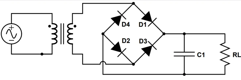
Bridge Rectifier Circuit Diagram
A complete bridge rectifier involves the following components:
1) An AC source that supplies the input AC waveform to the whole circuit. This is likely to be the grid (mains) electricity supplied by a wall outlet but may also be another AC source or a function generator.
2) A step-down transformer that brings the peak voltage to the desired level. The output of the step-down transformer is an AC waveform with the desired voltage.
3) Four diodes (D1, D2, D3, and D4) that rectify the AC and produce a pulsed DC output.
4) A resistive load RL, which simulates the circuit that the bridge rectifier is providing the power to.
The total output of the circuit, Vout, is measured across the load RL.
Bridge Rectifier Operation
How Does a Bridge Rectifier Work?
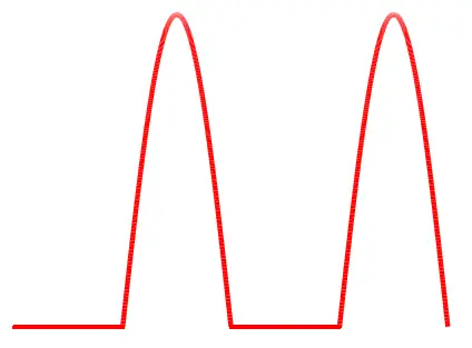
Direct current (DC) always flows in one direction, but alternating current (AC) flows in both directions in a sinusoidal pattern, called a waveform.
Both the voltage and current follow a sine-wave (sinusoidal) pattern.
The image on the right shows the waveform of 120V AC power in the US, which has a frequency of 60 Hz.
When the waveform is positive, the current is moving in the ‘forward’ direction.
When the waveform is negative, the current is moving in the ‘reverse’ direction.
This is why this type of current is called alternating current; the current alternates direction. Instead of electrons processing through a circuit, they wiggle back and forth in the opposite direction of conventional current.
In a bridge rectifier, two diodes rectify the AC waveform, ‘chopping off’ the bottom half wave of the AC signal and leaving only the top half wave.
The other two diodes are used to direct the current through the load and prevent a short circuit back to the transformer.
This results in a pulsed DC signal through the load.
There are two distinct stages of rectification with a bridge rectifier, with each stage corresponding to a half-cycle of the waveform.
First Half-Cycle
During the first half-cycle, the ‘top’ of the transformer’s secondary windings is positively biased and the ‘bottom’ is negatively biased. This means that current wants to flow from the top of the transformer to the bottom, clockwise through the circuit.
When the current reaches the junction between diodes D1 and D4, it can only pass through D1. D1 is active, allowing current to flow. D4 is also important, as it blocks a short circuit through D2 and back to the transformer.
The current flows through D1 and then through the load RL. It travels back to the diode bridge, where the negative potential at the bottom of the transformer pulls it through D2 and back to the transformer, completing the path.
Output of First Half-Cycle
The output of the first half-cycle is a pulsed DC output identical to the output of a half-wave rectifier.
This output features periods with a positive pulse and equal periods during which the output is zero (0).
Second Half-Cycle
During the second half-cycle, the bottom of the transformer is now positively biased and the top of the transformer is negatively biased. This means that current wants to flow from the bottom to the top, in a counter-clockwise fashion through the circuit.
Current leaves the bottom of the transformer and travels to the junction between D2 and D3 but it can only pass through D3. D2 prevents a short circuit back to the top of the transformer, forcing the current to travel through D3 and through the load.
The current travels through the load in the same direction as it did during the first half-cycle.
This is the ‘trick’ behind the bridge rectifier; the current always travels through the load in the same direction, thereby functioning as DC from the perspective of the load.
The current travels again to the junction between D2 and D4 but this time it is pulled by the negative potential at the top of the transformer, travelling up through D4 and completing the path.
The output of the second half-cycle is a waveform that is identical to the output of the first half-cycle, but phase shifted by 180 degrees.
This means that as D1 is pulsing, D2 is ‘off’. As D2 is pulsing, D1 is ‘off’.
Output of Second Half-Cycle
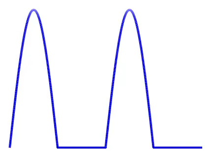
The output of D2 is then combined with the output of diode D1, forming a waveform with constant pulses:
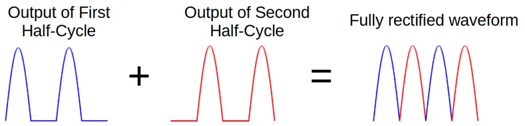
We can see that this output is identical to that of the full-wave rectifier.
Thus the elegant design of the bridge rectifier results in an output that would ordinarily require a transformer twice the size.
Bridge Rectifier Formula
The equivalent DC voltage output of a bridge rectifier is identical to that of the full-wave rectifier. It is the average value of the voltage pulse.
This can be found by using the peak voltage (Vpeak) in the following formula:
V_{DC} = \frac{2V_{peak}}{\pi}Note: You can find the derivation at the end of this tutorial if you’re interested.
However, the peak voltage isn’t exactly the peak of the AC voltage input. Each diode has a voltage drop called the forward voltage. For silicon-based diodes, the voltage drop is about .7 volts. So Vpeak is equal to the peak AC voltage minus the forward voltage of the diode:
V_{peak} = V_{ACpeak} -(2 \times .7V)=V_{ACpeak} - 1.4VTherefore the average DC output voltage can be related directly to the peak of the AC waveform:
V_{DC} = \frac{2(V_{ACpeak}-1.4V)}{\pi}Bridge Rectifier With Capacitor Filter
The bridge rectifier produces a higher quality output signal than the half-wave rectifier. However it still features pulses that decline all the way to zero and then rise back up the peak.
Like other rectifiers, the output of the full-wave rectifier can be significantly improved by adding a smoothing capacitor to the circuit.
Bridge Rectifier Capacitor Filter Circuit Diagram
The capacitor stores charge when the voltage is increasing during the ‘upward’ section of the wave. A corresponding voltage is generated across the capacitor.
When the voltage begins to decrease, the capacitor begins to act as a second voltage source, releasing the charge it has stored.
Instead of dropping to zero, the new waveform slowly declines from the peak voltage as the capacitor discharges.
Thus the capacitor buffers the total voltage measured across the load.
The capacitor then recharges during the next cycle, and the process begins again.
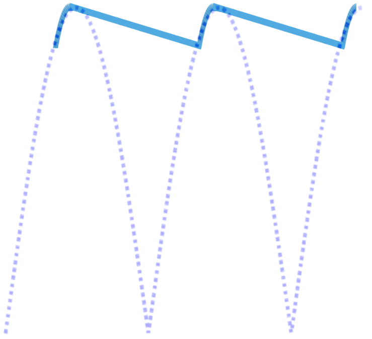
This results in a waveform that much more closely resembles an ideal DC signal, which would be a flat line.
Advantages and Drawbacks of Bridge Rectifiers
Bridge rectifiers are so common because they combine the main advantages of both half-wave and full-wave rectifiers.
However, the output of a bridge rectifier, even with a smoothing capacitor, is still not of a particularly high quality compared with a standard DC signal, which has a flat waveform.
For this reason, it is critical that more sophisticated filtering circuits are implemented in order to bring the output of the bridge rectifier to an acceptable quality for electronics.
In the next section, we’ll explore some of the most important filter circuits, starting with the L-filter.
Bridge Rectifier Formula Derivation
The calculation of the formula for the average output of the bridge rectifier is identical to that of the full-wave rectifier. So if you already read the tutorial on full-wave rectifiers, what follows will be a review.
The average value of any curve can be found by finding the area under the curve and dividing by the x-axis dimension over which we are trying to calculate the average.
In this case, we are trying to find the average value of the top half of a sine curve, which corresponds to the pulsed DC output of the half-wave rectifier.
Finding the area under a sine curve isn’t easy using traditional geometrical methods (dividing the curve up into tine rectangles).
Calculus provides a much easier way to find the area under the curve by calculating its’ integral. For example, in order to find the area of the sine wave between point a and point b in the figure, we can simply calculate the definite integral of sine (which is negative cosine) between points a and b:
\int_{a}^{b} \sin x \, dx = - \cos x \rvert_a^bWe scale this result to the value of the peak of the waveform by multiplying it by Vpeak:
Area = V_{peak} \int_{a}^{b} \sin{x} \, dx = -V_{peak} \cos{x}\rvert_{a}^{b}Point a and b are both located where the y-value of the curve (the voltage) is equal to zero. This corresponds with values of zero (0) and pi (π). So we need to evaluate the function between 0 and π:
Area = V_{peak} \int_{0}^{\pi} \sin{x} \, dx = -V_{peak} \cos{x}\rvert_{0}^{\pi}Now we just need to evaluate cosine at 0 and π and simplify:
Area = -V_{peak} \cos{x}\rvert_{0}^{\pi} = -V_{peak} [\cos \pi - \cos 0] = -V_{peak} [-1-1]=-V_{peak}[-2]=2V_{peak}So 2Vpeak is the area under the curve.
In order to calculate the average value, we simply divide this by the x-axis dimensional ‘length’ between points a and b. Point a is at zero and point b is at π so this is equal to π – 0, or π:
Average = \frac{2V_{peak}}{\pi - 0} = \frac{2V_{peak}}{\pi}Current in Bridge Rectifiers
We can derive the current in a bridge rectifier using the same procedure that we used for the half-wave rectifier.
We’ll start by noting that the current in a bridge rectifier varies periodically (like a sine wave) with the voltage.
Let’s use the term Vi to designate the voltage coming from the secondary windings of the transformer:
V_i = V_{m}\sin{2\pi ft}We can then use Ohm’s Law to derive the current, and we should note that the current will be limited by two types of resistance: (1) the load resistance RL, and (2) the forward resistance of the diode Rf. The forward resistance can be found by using the diode’s I-V characteristic.
I = \frac{V_i}{2R_f+R_L}=\frac{V_{m}}{2R_f+R_L}\sin{2\pi ft}We can also define a new term, Im, again using Ohm’s Law. This will help us simplify this equation a bit and aid in future calculations:
I_m = \frac{V_m}{2R_f+R_L}Therefore in terms of Im, the current is:
I = I_m \sin{2\pi ft}We can also define another helpful term, α, to simplify this equation even further:
\alpha =2\pi ft
Therefore the current is:
I = I_m \sin{\alpha}Note that all we’ve done is define the current as a sine wave, and use Im and α to simplify it.
RMS Current in Bridge Rectifier
Another important value is the root mean square (RMS) of the current. The RMS is the square root of the mean, squared (to the second power):
I_{rms} = \sqrt{\frac{1}{2\pi}\int_0^{2\pi}I^2 \,d\alpha}Not that the factor of 1/2π in front of the integral is used because we are taking the average value over the range of 0 to 2π.
Therefore the value of Irms2 is equal to:
I_{rms}^2 = \frac{1}{2\pi}\int_0^{2\pi}I^2 \,d\alpha = \frac{1}{2\pi}\int_0^{\pi} I_m^2 \sin^2{\alpha} \,d\alphaWhere the term from π to 2π goes to zero because the current is zero for the second half-cycle.
Simplifying this, we find:
I_{rms}^2 = \frac{I_m^2}{2}Therefore the RMS current is:
I_{rms} = \frac{I_m}{\sqrt2}Form Factor of Bridge Rectifier
The form factor (abbreviated by f) is a quantity used to help compare the RMS and average values of a function.
It is defined as the ratio of the RMS current over the average current:
f=\frac{I_{rms}}{I_{DC}} = \frac{\frac{I_m}{\sqrt{2}}}{\frac{2I_m}{\pi}} =\frac{\pi}{2\sqrt{2}} \approx 1.1107Bridge Rectifier AC Output
The total output current can be divided into a DC component and an AC component. The DC component is identical to the average value over the whole waveform, IDC, and we can express that AC component as I’.
I = I_{DC} + I'Where I’ represents the AC component of the output waveform.
It turns out that the RMS of I’ is an important factor in its’ own right.
We can define I’ as the difference between the total current and the DC component of the current:
I' = I-I_{DC}We can then find the RMS value of I’ by calculating the square root of the square of its’ mean:
I_{rms}' = \sqrt{\frac{1}{2\pi}\int_0^{2\pi}I'^2 \,d\alpha} = \sqrt{\frac{1}{2\pi}\int_0^{2\pi}(I-I_{DC})^2 \,d\alpha} Just as we did earlier, we can simplify this by squaring both sides:
I_{rms}'^{2} = \frac{1}{2\pi}\int_0^{2\pi}(I-I_{DC})^2 \,d\alpha = \frac{1}{2\pi}\int_0^{2\pi}I^2-2I(I_{DC})+I_{DC}^2 \,d\alphaThis can be divided into three individual terms. The first is identical to I2rms the second simplifies to -2I2DC and the third simplifies to I2DC.
In other words,
I_{rms}'^{2} = I_{rms}^2 - 2I^2_{DC} +I_{DC}^2 = I_{rms}^2 - I_{DC}^2Therefore the RMS of the AC component is:
I_{rms}' = \sqrt{I_{rms}^2 - I_{DC}^2}Bridge Rectifier Ripple Factor
Now that we have quantified the AC component of the bridge rectifier, we can compare it’s RMS value with the RMS value of the DC component.
This ratio is called the ripple factor, which helps us to understand the magnitude of the AC component compared with the magnitude of the DC component.
The ripple factor is abbreviated by the Greek letter gamma (γ):
\gamma = \frac{I_{rms}'}{I_{DC}}Using the values we found earlier, we can write the ripple factor of the full-wave rectifier as:
\gamma=\frac{\sqrt{I_{rms}^2-I_{DC}^2}}{I_{DC}}=\sqrt{(\frac{I_{rms}}{I_{DC}})^2-1}=\sqrt{f^2-1}=\sqrt{(\frac{\pi}{2\sqrt2})^2-1} \approx 0.483A high ripple factor indicates that the signal still has a large AC component, indicating that the resulting current is far from an ideal DC signal.
Efficiency of Bridge Rectifier
The efficiency of the circuit is the measure of its’ power output to its’ power input. Efficiency is abbreviated by the Greek letter eta (η).
To calculate the efficiency, we must find the output power of both the DC and AC components of the output waveform. In other words,
\eta = \frac{P_{O,DC}}{P_{in}}Where PO,DC is the output DC power and Pin is the input power.
For the DC component, the output power is given by the I2R formula:
P_{O,DC} = I_{DC}V_{DC}=I_{DC}I_{DC}R_L=I_{DC}^2R_LFor the input, we use the relation P = VI:
P_i = V_i \times I = V_m\sin{\alpha}\times I_m\sin{\alpha}=V_mI_m\sin^2{\alpha}This is the formula for the instantaneous power at a specific value of α; to find the total power, we must integrate:
P_{in}=\frac{1}{2\pi}\int_0^{2\pi}P_i\,d\alphaSubstituting Pi, we find:
P_{in}=\frac{1}{2\pi}\int_0^{\pi}V_mI_m\sin^2{\alpha}\,d\alphaNoting again that the π to 2π component is again zero as the current is zero.
Recall the definition of Vm:
V_m=I_m(2R_f+R_L)
We now substitute this into the equation for Pin:
P_{in}=\frac{1}{2\pi}I_m^2(2R_f+R_L)\int_0^{\pi}\sin^2{\alpha}\,d\alphaRecall the our formula for Irms from earlier:
I_{rms}^2=\frac{1}{2\pi}\int_0^{\pi} I_m^2 \sin^2{\alpha} \,d\alphaWhich we can use to simplify Pin:
P_{in}=I_{rms}^2(2R_f+R_L)We can now solve for the efficiency of the half-wave rectifier:
\eta=\frac{I_{DC}^2R_L}{I_{rms}^2(R_f+R_L)}Substituting the known values for IDC and Irms:
\eta=\frac{\frac{4I_m^2}{\pi^2}}{\frac{I_m^2}{2}}\frac{R_L}{2R_f+R_L}=\frac{8}{\pi^2}\frac{R_L}{2R_f+R_L}=0.81\frac{R_L}{2R_f+R_L}Thus we can see that the maximum possible efficiency of the half-wave rectifier is 81%. This is twice the efficiency of the half-wave rectifier.
Full-Wave Rectifier Transformer Utilization Factor (TUF)
The transformer utilization factor is the ratio of DC output power to the AC power rating of the secondary winding.
Mathematically, this can be written as:
TUF = \frac{P_{o,DC}}{V_{RMS}\times I_{RMS}}The DC power output can be found by using the I2R formula:
P_{o,DC}=I_{DC}^2R_L=\frac{4I_m^2}{\pi^2}R_LThe RMS value of a full sine wave is the peak value of the wave divide by the square root of two (2), so we can state that VRMS must be equal to:
V_{RMS} = \frac{V_m}{\sqrt{2}} = \frac{I_m(2R_f+R_L)}{\sqrt{2}}We have previously found that the RMS value for the current for the half-wave (IRMS) is:
I_{RMS} = \frac{I_m}{\sqrt2}Thus the transformer utilization factor is:
TUF = \frac{4I_m^2}{\pi^2}\frac{R_L}{\frac{I_m}{\sqrt{2}}\frac{I_m}{\sqrt2}(2R_f+R_L)}=\frac{8}{\pi^2}\frac{R_L}{2R_f+R_L}=0.81\frac{R_L}{R_f+R_L}Therefore the maximum transformer utilization factor for the full-wave rectifier is 81%.
Bridge Rectifier Peak Inverse Voltage (PIV)
When constructing a bridge rectifier, the peak inverse voltage must be taken into account because the diodes must be chosen so that their breakdown voltage is greater than the PIV.
The PIV is equal to the maximum voltage Vm:
PIV=V_m
Therefore the diode must be chosen so that the breakdown voltage VBR is greater than Vm:
V_{BR} > V_m