Electric Field

An electric field is a non-contact force field that extends out from every charged particle, causing a force on other charged particles.

In our last lesson (electric charge), we learned that electric charges exert an attractive or repulsive force on each other. This force is called the electromagnetic force and is what holds atoms together by keeping electrons bound to the protons in the nucleus. The electromagnetic force also prevents atoms from collapsing into each other due to the mutual repulsion of electrons in different atoms.

How is it that charged particles can exert a force on each other from a distance (i.e. without touching)?

The answer is that electric charge results in an electric field that extends out into the space around the particle.

The total force of an electric field increases with the amount of charge (number of charged particles) in an object, and decreases with distance from the object.

Coulomb’s Law

In the 1780’s, French physicist Charles Coulomb set about investigating the nature of the forces exchanged between charged objects. His result was an equation that mathematically describes the force from a charged object on another.

This is called Coulomb’s Law:

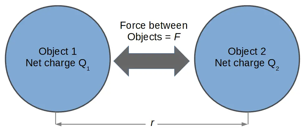
F = k\frac{Q_1Q_2}{r^2}

Where Q₁ and Q₂ represent the net electric charge on object 1 and object 2, respectively, and r is the distance between them.

We can see that the basic relation described by Coulomb’s law is that the force is proportional to the amount of electric charge in each object, and inversely proportional to the square of the distance between them.

There is also a constant of proportionality ‘k‘ called Coulomb’s constant. The constant k is there to make the SI units work correctly during calculations. Coulomb’s constant k has the following value:

k = 8.99 \times 10^9 N\frac{m^2}{C^2}

If both objects have either a positive or negative charge, then the total force between them will be positive, indicating a repulsive force.

If one object has a positive charge and the other has a negative charge, then the total force between them will be negative, indicating an attractive force.

Inverse-Square Law

One of the most interesting things about Coulomb’s law is that it is a prominent example of an inverse-square law. This means that the force is reduced by the square of the distance between the objects.

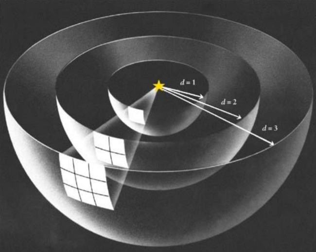
Inverse square laws occur because of the geometric dilution of the force over space. If we were to draw a sphere around a charged particle, we would find that as we increase the distance from the charge, the surface area of the sphere increases. Thus at any given point on the sphere, the intensity of the electric field decreases.

The image on the right shows a good example of this. On the inner sphere (d=1), the field only occupies one surface square. A bit further out at d=2, the same ‘strength’ of the field now occupies four squares; it’s strength has been diluted by 4x so the field strength of any one square is only 1/4 as strong as it was at d=1. Still farther out, out d=3, the same field now occupies nine squares so the field strength of any square is now 1/9 as strong as a square on the d=1 surface.

This could be predicted by noticing that the square of 2 is 4 and the square of 3 is 9. If we wanted to predict the relative field strength at, for example, d = 2.3, we can just square this value and take the inverse:

d = 2.3 => Strength = \frac{1}{(2.3)^2} = \frac{1}{5.29}

Thus at d = 2.3, the strength of the field is only 1/5.29 its’ strength at d = 1.

Electric Field and Gravitational Field Similarity

Gravity is another inverse-square law, and it is notable that its’ form is very similar to Coulomb’s law:

F_g = G\frac{M_1M_2}{r^2}

Notice that if we were to substitute the masses M₁ and M₂ for charges Q₁ and Q₂, and replace the gravitational constant G with Coulomb’s constant k, we would in fact have Coulomb’s law.

Coulomb’s Law and Electric Field

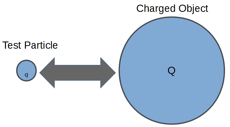
The electric field of a charged object can be directly related to Coulomb’s law by using a test particle. A test particle is simply a small particle with a charge of q that is used to ‘test’ the field of a larger charged object nearby.

Coulomb’s Law for a Test Particle

Using Coulomb’s Law to determine the force between charged objects, we can define the electric field of a charged object with charge Q by using a small test particle with charge q.

In this case, we will use Coulomb’s law and substitute the charge value q for the charge of object 1, Q₁. We can also rename Q₂ (the charge of object 2) to Q to simplify the equation further. In any case, this equation is fully equivalent to the above definition of Coulomb’s Law. We are just renaming the charge values to make things more clear.

The resulting force is then:

F = k \frac{Q_1Q_2}{r^2} = k \frac{qQ}{r^2}

Which is the force ‘F‘ between a test charge q and another object with charge Q, at distance r.

The Electric Field

The electric field can now be mathematically defined as the force exerted on the test charge, divided by the value of the test charge.

In other words, the electric field is the force per unit charge.

The value of the electric field is abbreviated by an uppercase ‘E’:

E = \frac{F}{q}

If we substitute the value of the force from Coulomb’s Law, we obtain the following:

E = \frac{F}{q}=k\frac{qQ}{qr^2}

The charge value of the test charge (q) cancels in the numerator and denominator to give our final result:

E = k\frac{Q}{r^2}

So the electric field of a charged object is proportional to the charge of the object divided by the square of the distance from the object.

Electric Field Lines

It can be useful to be able to visualize electric fields in order to better understand them.

Electric fields can be graphically depicted as lines extending into or away from the charged object.

Arrows on the lines indicate the direction that a positive test charge would move if it were placed in the electric field.

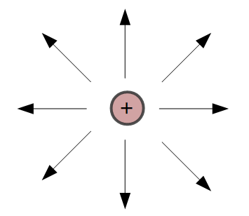
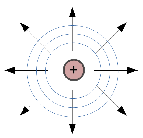
Positively charged objects have field lines pointing away from the surface of the object.

Notice in the figure on the right, the arrows are pointing away from the positive charge, indicating that a positive charge placed in this field would be repelled by the object.

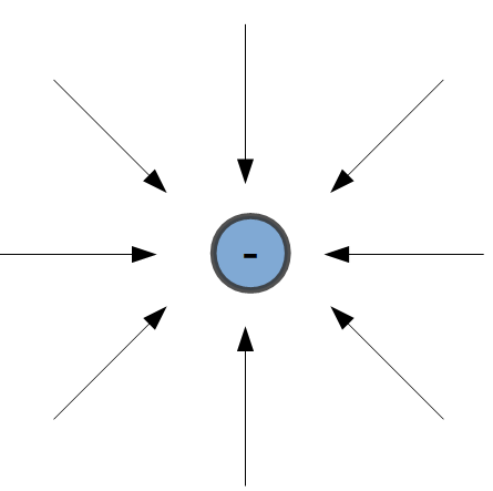
Negatively charged objects have field lines pointing into the surface of the object. The figure on the left shows arrows pointing into the electric charge.

In this case, the arrows indicate that a positive test charge would be attracted to the center of the negative charge.

In each case, the strength, or magnitude, of the field is determined by the distance from the surface of the object. The blue circles on the image to the right indicate that the field strength is the same at each point on the circle. These circles are also called equipotential lines.

When charged objects are placed near each other, their field lines combine to make really interesting patterns. The best way to understand field lines is to use a simulator.

University of Colorado PhET Charges and Fields Simulation

The University of Colorado has created an amazing simulation to help visualize electric charges and fields. It’s part of their free PhET interactive simulations program.

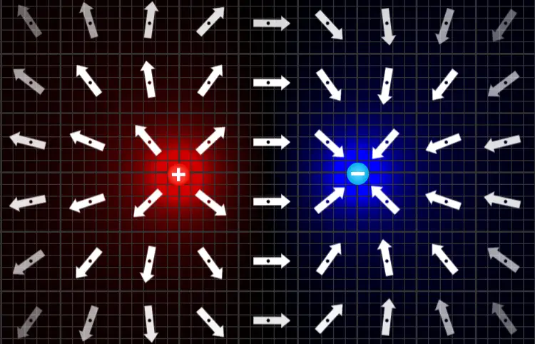
To use the simulator, just grab a positive or negative charge and drop it into the field. You can combine lots of different charges in interesting ways to see the combined effect on the electric field. On the right is a screenshot in which we used the simulator to visualize the electric field of a positive charge next to a negative charge.

The strength of the electric field is represented by the transparency of the arrows. The arrows at the corners are more transparent because the field is weasest at the farthest distances from the charges.

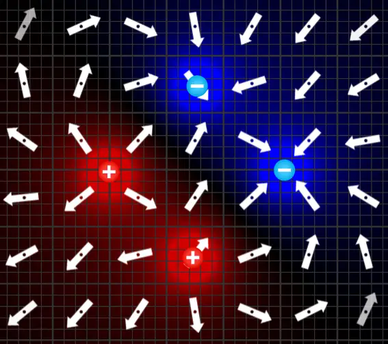
Here’s an image of a more complex field created by two positive charges and two negative charges. The combinations are endless with this simulator!

You can find the simulation here or use the embedded simulator below:

Note: Sometimes the simulator doesn’t pre-load with this webpage. If the simulator isn’t already loaded, try right-clicking and pressing ‘reload’ or reload the page.

Electric Field and Charge

We previously defined electric charge as the property of matter that causes a charged object to experience a force due to the presence of another charged object.

With this definition in mind, we can see that electric fields are the reason charges exert a force on each other.

In other words, an electric charge exhibits an electric field that exerts a force on other charges.

The concepts of electric charge and field are thereby interlinked with each other.

Module 1 Complete

You have completed the first module and should have a good grounding in basic concepts related to electricity. If this was your first introduction to many of these topics, we recommend re-reading sections as they will become more clear over time. Reviewing the beginning of Module 2, in particular the sections on Current and Voltage, will also help you to better understand the information presented in Module 1.

In the Module 2, we will build on what we’ve learned to explore DC circuits. By the end, you’ll have a solid grounding in basic DC theory including voltage, current, resistance, and capacitance, and will be able to understand and read electrical schematics for a variety of DC circuits.

Let’s get on with the show at Module 2’s Introduction: Introduction to Module 2