Half-Wave Rectifier
Rectifiers are circuits that turn an alternating current (AC) into a direct current (DC). Rectifiers are incredibly useful in the field of electronics because most electronic devices use DC, but the power grid (mains electricity) supplies AC. The three most common types are the half-wave rectifier, the full-wave rectifier, and the bridge rectifier.
A half-wave rectifier is a circuit that allows only one half of an alternating current (AC) waveform to pass, turning an AC signal into a pulsed direct current (DC) signal.
Half-wave rectifiers are the simplest type of rectifier, and are the perfect starting point for learning about rectifiers in general.
The following table provides a comparison of each type of rectifier.
| Type | Number of Diodes | Transformer Type | Output |
| Half-Wave Rectifier | 1 | Normal | Half-wave |
| Full-Wave Rectifier | 2 | Center Tapped | Full-wave |
| Bridge Rectifier | 4 | Normal | Full-wave |
- Half-Wave Rectifier Circuit
- Half Wave Rectifier Operation
- Half-Wave Rectifier Formula
- Half-Wave Rectifier With Capacitor Filter
- Drawbacks of Half-Wave Rectifiers
- Mathematical Analysis of Half-Wave Rectifiers
- Current in Half-Wave Rectifier
- Half-Wave Rectifier Formula Derivation
- Average Current in Half-Wave Rectifier
- RMS Current in Half-Wave Rectifier
- Form Factor of Half-Wave Rectifier
- Half-Wave Rectifier AC Output
- Half-Wave Rectifier Ripple Factor
- Efficiency of Half-Wave Rectifier
- Half-Wave Rectifier Transformer Utilization Factor (TUF)
- Full-Wave Rectifier Peak Inverse Voltage (PIV)
Half-wave rectifiers use only one single diode, and are the simplest way to convert AC into DC. They are cheap and easy to make but are inefficient because only half of the AC waveform is used; the other half goes to waste.
Half wave rectifiers are ‘building blocks’ for more complex rectifier circuits like full wave rectifiers and bridge rectifiers. Their simplicity makes them an ideal starting point for learning how rectifiers work.
Half-Wave Rectifier Circuit
At the heart of a half-wave rectifier is a single diode. As we’ve learned, the function of a diode is to allow electric current to flow in only one direction, based on the operation of a p-n junction. Current in the diode flows from the anode to the cathode, as shown below:

Current can only flow from the anode to the cathode; it can’t flow in the reverse direction without harming the diode.
Note: There are some diodes that are designed to allow reverse current (Zener diodes), but they aren’t used in rectifiers.
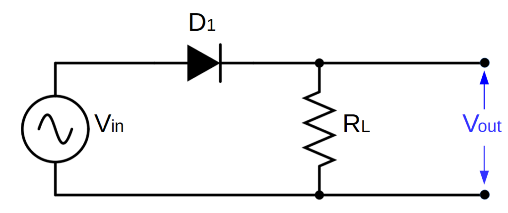
A simple half wave rectifier is a diode connected with an AC voltage source (Vin) and some type of resistive load (RL), as shown below:
Half-Wave Rectifier Circuit Diagram
The output of the circuit, Vout, is measured across the load RL.
Since a diode only allows current to flow in one direction, when it is co nnected with an alternating current (AC), it will only allow the ‘positive’ current to pass. This produces a type of DC current known as pulsed DC.
Therefore, a half wave rectifier converts an alternating current signal into a pulsed direct current signal. This is where they get their name from: half wave rectifiers only allow one half of the AC waveform to pass.
Another common presentation of a half-wave rectifier circuit adds a step-down transformer to the circuit, which decreases the voltage to a more suitable level (most commonly for use in electronics) before rectifying the AC into DC.
Half-Wave Rectifier With Step-Down Transformer
This step is important as transformers can only be used with AC (i.e. transformers don’t work with DC). It’s easier and more efficient to first bring the voltage down to a useable level and then rectify it than it is to rectify and then try and reduce the voltage.
Note that the transformer isn’t really integral to the operation of the rectifier; it’s just a logical pre-rectification step.
Half Wave Rectifier Operation
How Does a Half Wave Rectifier Work?
Half wave rectifiers rely on the fact that AC travels in both directions, but diodes only allow current to travel in one direction.
Direct current (DC) always flows in one direction, but alternating current (AC) flows in both directions in a sinusoidal pattern, called a waveform.
The image on the right shows the waveform of 120V AC power in the US, which has a frequency of 60 Hz.
When the waveform is positive, the current is moving in the ‘forward’ direction.
When the waveform is negative, the current is moving in the ‘reverse’ direction.
This is why this type of current is called alternating current; the current alternates direction. Instead of electrons processing through a circuit, they wiggle back and forth in the opposite direction of conventional current.
The diode in a half-wave rectifier is used to allow only the positive current from an AC source to flow.
The diode is used to remove the negative part of the AC waveform, ‘chopping off’ the bottom half wave of the AC signal and leaving only the top half wave.
This results in a pulsed DC signal that retains only the positive part of the AC waveform.
In the pulsed DC output of the half-wave rectifier, current always moves in the same direction, but increases and decreases over time, with periods of zero (0) current in between pulses.
While we have successfully used a diode to convert AC into DC, this type of pulsed signal is not as useful as a standard DC signal, which provides a constant output.
Half-Wave Rectifier Formula
The equivalent DC voltage output of a half-wave rectifier is the average value of the voltage pulse.
This can be found by using the peak voltage (Vm) in the following formula:
V_{DC} = \frac{V_{m}}{\pi}Note: Deriving this formula requires some calculus. You can find the derivation below if you’re interested.
However, the peak voltage isn’t exactly the peak of the AC voltage input. The diode has a voltage drop called the forward voltage. For silicon-based diodes, the voltage drop is about .7 volts. So Vpeak is equal to the peak AC voltage minus the forward voltage of the diode:
V_{m} = V_{ACpeak} - .7 VTherefore the average DC output voltage can be related directly to the peak of the AC waveform:
V_{DC} = \frac{V_{m}}{\pi}=\frac{V_{ACpeak}-.7V}{\pi}Half-Wave Rectifier With Capacitor Filter
A half-wave rectifier successfully converts an AC source into a DC output, but the half-sine wave pulsations are often undesired. The most commonly used DC sources are steady-state, meaning that the goal of rectification is a flat line rather than a pulsed sine wave.
The output of the half-wave rectifier can be dramatically improved with the simple addition of a smoothing capacitor as shown below:
Half Wave Rectifier Capacitor Filter Circuit Diagram
The capacitor stores charge when the voltage is increasing during the ‘upward’ section of the wave. A corresponding voltage is generated across the capacitor.
When the voltage begins to decrease, the capacitor begins to act as a second voltage source, releasing the charge it has stored.
Instead of dropping to zero, the new waveform slowly declines from the peak voltage as the capacitor discharges.
Thus the capacitor buffers the total voltage measured across the load.
The capacitor then recharges during the next cycle, and the process begins again.
This results in a waveform that much more closely resembles an ideal DC signal, which would be a flat line.
Drawbacks of Half-Wave Rectifiers
Half-wave rectifiers are the simplest and cheapest method for converting AC into DC. But they have some major drawbacks that reduce the benefit of using them in real devices.
First, half-wave rectifiers are very inefficient. By cutting out the negative half of the input AC source, they lose half of the potential power that is supplied at the output. A 50% loss is extreme, especially when the primary job of the circuit is to convert AC into DC as efficiently as possible.
Second, the output waveform of a half-wave rectifier is fairly poor. Even with a capacitor, the voltage drops off significantly between each peak. This could easily cause electronics including logic circuits to malfunction.
While we could in theory work with the limitations of a half-wave rectifier, it turns out that by adding just a little more complexity and a little more cost, we can significantly improve on both of these issues.
If we add just one more diode, we can turn the half-wave rectifier into a full-wave rectifier. A full wave rectifier is twice as efficient and produces a higher quality waveform than the half-wave rectifier. Considering that diodes cost only a few cents, this improvement is easily worth the added cost and complexity.
Mathematical Analysis of Half-Wave Rectifiers
The following topics will cover slightly more advanced topics of half-wave rectifiers like current, ripple factor and transformer utilization factor (TUF). While these topics are not crucial for a basic understanding of half-wave rectifiers, they are useful for gaining a high level of working knowledge.
Current in Half-Wave Rectifier
The current in a half-wave rectifier varies periodically with the voltage.
Let’s use the term Vi to designate the voltage coming from the secondary windings of the transformer:
V_i = V_{m}\sin{2\pi ft}We can use Ohm’s Law to derive the current, and we should note that the current will be limited by the load resistance RL as well as the forward resistance of the diode Rf.
I = \frac{V_i}{R_L+R_f}=\frac{V_{m}}{R_f+R_L}\sin{2\pi ft}Note that this applies only to the first half cycle; the current in the second half cycle is zero because the diode is reverse biased.
We can also define a new term, Im, that will help us simplify this equation a bit and help us in future calculations:
I_m = \frac{V_m}{R_f+R_L}Therefore in terms of Im, the current is:
I = I_m \sin{2\pi ft}We can also define another helpful term, α, to simplify this equation even further:
\alpha =2\pi ft
Therefore the current is:
I = I_m \sin{\alpha}Half-Wave Rectifier Formula Derivation
The average value of any curve can be found by finding the area under the curve and dividing by the x-axis dimension over which we are trying to calculate the average.
In this case, we are trying to find the average value of the top half of a sine curve, which corresponds to the pulsed DC output of the half-wave rectifier.
Finding the area under a sine curve isn’t easy using traditional geometrical methods (dividing the curve up into tine rectangles).
Calculus provides a much easier way to find the area under the curve by calculating its’ integral. For example, in order to find the area of the sine wave between point a and point b in the figure, we can simply calculate the definite integral of sine (which is negative cosine) between points a and b:
\int_{a}^{b} \sin x \, dx = - \cos x \rvert_a^bWe scale this result to the value of the peak of the waveform by multiplying it by Vpeak:
Area = V_{m} \int_{a}^{b} \sin{x} \, dx = -V_{m} \cos{x}\rvert_{a}^{b}Point a and b are both located where the y-value of the curve (the voltage) is equal to zero. This corresponds with values of zero (0) and pi (π). So we need to evaluate the function between 0 and π:
Area = V_{m} \int_{0}^{\pi} \sin{x} \, dx = -V_{m} \cos{x}\rvert_{0}^{\pi}Now we just need to evaluate cosine at 0 and π and simplify:
Area = -V_{m} \cos{x}\rvert_{0}^{\pi} = -V_{m} [\cos \pi - \cos 0] = -V_{m} [-1-1]=-V_{peak}[-2]=2V_{m}So 2Vpeak is the area under the curve.
In order to calculate the average value (which we’ll call VDC), we simply divide this by the x-axis dimensional ‘length’ between points a and b. Point a is at zero and point b is at π so this is equal to π – 0, or π:
V_{DC}= \frac{2V_{m}}{\pi - 0} = \frac{2V_{m}}{\pi}However because we are dealing with a half wave, there is also a period after the pulse where the voltage is equal to zero. This period is equal to the period of the pulse itself so the mathematically we must double the value of the denominator (or use an x-axis ‘length’ from 0 to 2π):
V_{DC} = \frac{2V_{m}}{2 \pi - 0} = \frac{V_{m}}{\pi}Average Current in Half-Wave Rectifier
The above analysis can be applied to find the average value of the current as well.
The only difference is that because we are solving for current, we use the term Im instead of Vm.
Therefore,
I_{DC} = \frac{I_m}{\pi}RMS Current in Half-Wave Rectifier
Another important value is the root mean square (RMS) of the current. The RMS is the square root of the mean, squared (to the second power):
I_{rms} = \sqrt{\frac{1}{2\pi}\int_0^{2\pi}I^2 \,d\alpha}Not that the factor of 1/2π in front of the integral is used because we are taking the average value over the range of 0 to 2π.
Therefore the value of Irms2 is equal to:
I_{rms}^2 = \frac{1}{2\pi}\int_0^{2\pi}I^2 \,d\alpha = \frac{1}{2\pi}\int_0^{\pi} I_m^2 \sin^2{\alpha} \,d\alphaWhere the term from π to 2π goes to zero because the current is zero for the second half-cycle.
Simplifying this, we find:
I_{rms}^2 = \frac{I_m^2}{4}Therefore the RMS current is:
I_{rms} = \frac{I_m}{2}Form Factor of Half-Wave Rectifier
The form factor (abbreviated by f) is a quantity used to help compare the RMS and average values of a function.
It is defined as the ratio of the RMS current over the average current:
f=\frac{I_{rms}}{I_{DC}} = \frac{\frac{I_m}{2}}{\frac{I_m}{\pi}} =\frac{\pi}{2} \approx 1.571Half-Wave Rectifier AC Output
The total output current can be divided into a DC component and an AC component. The DC component is identical to the average value over the whole waveform, IDC, and we can express that AC component as I’.
I = I_{DC} + I'Where I’ represents the AC component of the output waveform.
It turns out that the RMS of I’ is an important factor in its’ own right.
We can define I’ as the difference between the total current and the DC component of the current:
I' = I-I_{DC}We can then find the RMS value of I’ by calculating the square root of the square of its’ mean:
I_{rms}' = \sqrt{\frac{1}{2\pi}\int_0^{2\pi}I'^2 \,d\alpha} = \sqrt{\frac{1}{2\pi}\int_0^{2\pi}(I-I_{DC})^2 \,d\alpha} Just as we did earlier, we can simplify this by squaring both sides:
I_{rms}'^{2} = \frac{1}{2\pi}\int_0^{2\pi}(I-I_{DC})^2 \,d\alpha = \frac{1}{2\pi}\int_0^{2\pi}I^2-2I(I_{DC})+I_{DC}^2 \,d\alphaThis can be divided into three individual terms. The first is identical to I2rms the second simplifies to -2I2DC and the third simplifies to I2DC.
In other words,
I_{rms}'^{2} = I_{rms}^2 - 2I^2_{DC} +I_{DC}^2 = I_{rms}^2 - I_{DC}^2Therefore the RMS of the AC component is:
I_{rms}' = \sqrt{I_{rms}^2 - I_{DC}^2}Half-Wave Rectifier Ripple Factor
Now that we have quantified the AC component of the half-wave rectifier, we can compare it’s RMS value with the RMS value of the DC component.
This ratio is called the ripple factor, which helps us to understand the magnitude of the AC component compared with the magnitude of the DC component.
The ripple factor is abbreviated by the Greek letter gamma (γ):
\gamma = \frac{I_{rms}'}{I_{DC}}Using the values we found earlier, we can write this as:
\gamma=\frac{\sqrt{I_{rms}^2-I_{DC}^2}}{I_{DC}}=\sqrt{(\frac{I_{rms}}{I_{DC}})^2-1}=\sqrt{f^2-1}=\sqrt{(\frac{\pi}{2})^2-1} \approx 1.21A high ripple factor indicates that the signal still has a large AC component, indicating that the resulting current is far from an ideal DC signal.
Efficiency of Half-Wave Rectifier
The efficiency of the circuit is the measure of its’ power output to its’ power input. Efficiency is abbreviated by the Greek letter eta (η).
To calculate the efficiency, we must find the output power of both the DC and AC components of the output waveform. In other words,
\eta = \frac{P_{O,DC}}{P_{in}}Where PO,DC is the output DC power and Pin is the input power.
For the DC component, the output power is given by the I2R formula:
P_{O,DC} = I_{DC}V_{DC}=I_{DC}I_{DC}R_L=I_{DC}^2R_LFor the input, we use the relation P = VI:
P_i = V_i \times I = V_m\sin{\alpha}\times I_m\sin{\alpha}=V_mI_m\sin^2{\alpha}This is the formula for the instantaneous power at a specific value of α; to find the total power, we must integrate:
P_{in}=\frac{1}{2\pi}\int_0^{2\pi}P_i\,d\alphaSubstituting Pi, we find:
P_{in}=\frac{1}{2\pi}\int_0^{\pi}V_mI_m\sin{\alpha}\,d\alphaNoting again that the π to 2π component is again zero as the current is zero.
Recall the definition of Vm:
V_m=I_m(R_f+R_L)
We now substitute this into the equation for Pin:
P_{in}=\frac{1}{2\pi}I_m^2(R_f+R_L)\int_0^{\pi}\sin^2{\alpha}\,d\alphaRecall the our formula for Irms from earlier:
I_{rms}^2=\frac{1}{2\pi}\int_0^{\pi} I_m^2 \sin^2{\alpha} \,d\alphaWhich we can use to simplify Pin:
P_{in}=I_{rms}^2(R_f+R_L)We can now solve for the efficiency of the half-wave rectifier:
\eta=\frac{I_{DC}^2R_L}{I_{rms}^2(R_f+R_L)}Substituting the known values for IDC and Irms:
\eta=\frac{\frac{I_m^2}{\pi^2}}{\frac{I_m^2}{2^2}}\frac{R_L}{R_f+R_L}=\frac{4}{\pi^2}\frac{R_L}{R_f+R_L}=.405\frac{R_L}{R_f+R_L}Thus we can see that the maximum possible efficiency of the half-wave rectifier is 40.5%.
Half-Wave Rectifier Transformer Utilization Factor (TUF)
The transformer utilization factor is the ratio of DC output power to the AC rating of the secondary winding.
Mathematically, this can be written as:
TUF = \frac{P_{o,DC}}{V_{RMS}\times I_{RMS}}The DC power output can be found by using the I2R formula:
P_{o,DC}=I_{DC}^2R_LThe RMS value of a full sine wave is the peak value of the wave divide by the square root of two (2), so we can state that VRMS must be equal to:
V_{RMS} = \frac{V_m}{\sqrt{2}} = \frac{I_m(R_f+R_L)}{\sqrt{2}}We have previously found that the RMS value for the current for the half-wave (IRMS) is:
I_{RMS} = \frac{I_m}{2}Thus the transformer utilization factor is:
TUF = \frac{I_{DC}^2R_L}{2\times\frac{I_m}{\sqrt{2}}\frac{I_m}{2}(R_f+R_L)}= \frac{4\times I_m^2}{\pi^2}\frac{R_L}{2\times \frac{I_m}{\sqrt{2}}\frac{I_m}{2}(R_f+R_L)}=\frac{4\sqrt{2}}{\pi^2}\frac{R_L}{R_f+R_L}=0.574\frac{R_L}{R_f+R_L}Therefore the maximum transformer utilization factor for the full-wave rectifier is .574.
Full-Wave Rectifier Peak Inverse Voltage (PIV)
When constructing a full-wave rectifier, the peak inverse voltage (PIV) must be taken into account because the diodes must be chosen so that their breakdown voltage is greater than the PIV.
The PIV is equal to the maximum voltage Vm:
PIV=V_m
Therefore the diode must be chosen so that the breakdown voltage VBR is greater than Vm:
V_{BR} > V_m